Designing more efficient quantum circuits with Claude

www.anthropic.com

Quantum computers will need carefully designed circuits to run useful algorithms on limited hardware. We gave Claude plain-language specifications for eight such circuits, drawn from chemistry, optimization, physics simulation, and number theory, along with an automated evaluator that checks and scores each design. Working largely on its own, Claude found designs that improve on the best published circuits, in some cases by an order of magnitude or more. Such improvements substantially reduce the quantum resources that useful applications require, so practical quantum computers could arrive sooner than previously anticipated.

This work was led by Andi Gu as part of Anthropic’s STEM Fellows Program, with mentorship from Alek Kemeny, a quantum physicist at Anthropic, in collaboration with Susanne Yelin (Harvard University) and Mikhail Lukin (Harvard University and QuEra Computing). Read the full paper on arXiv.

Unlike classical computers, which store information in bits whose value is either 0 or 1, quantum computers store information in qubits, which can be built from single atoms, superconducting circuits, or particles of light. These qubits make use of quantum phenomena such as superposition—which allows a quantum system to exist in a combination of states at once—in order to process information in ways that could make certain problems in fields like chemistry, materials science, and number theory tractable, even when they are too hard for traditional computers.

The quantum computers the field has built to date only have hundreds to thousands of qubits—too few to run many of the algorithms that promise practical advantages over classical computers. And these qubits are highly sensitive to environmental noise, such as heat, vibration, and even cosmic rays. A tiny disturbance can nudge a qubit’s state, and these small errors pile up until the computer gives the wrong answer.

Given that both qubits and computing time are scarce resources, researchers have been working to redesign quantum algorithms to use fewer qubits and complete computations in less time. An illustrative example is simulating FeMoco, the iron–sulfur cluster at the heart of nitrogenase, the enzyme that bacteria use to turn nitrogen from the air into ammonia. Understanding how it works could help scientists design better industrial catalysts—the substances manufacturers use to speed up chemical reactions.

In 2017, researchers estimated that a quantum computer would need about 50 trillion Toffoli gates to compute FeMoco’s ground-state energy—the energy of its most stable configuration, which chemists need in order to predict how FeMoco reacts. (Similar to ordinary computers, quantum computers work by applying a long sequence of simple operations, called gates, to their qubits. The Toffoli gate is one of the most expensive gates to run, so counting Toffoli gates is a standard way to estimate how long a computation will take.)

Through a series of algorithmic advances, the estimated number of gates has come down to about 340 million—a roughly 150,000-fold reduction, corresponding to a few hours of computation on a future machine with about three million physical qubits.1

These reductions largely came from redesigning the circuits that carry out the computation, rather than from making better hardware. Claude has proven particularly adept at optimizing classical algorithms, so we wanted to see whether it could do the same for quantum algorithms if it were given only a plain-language description of what each circuit must compute.

Claude is unusually well suited to this task, for several reasons. First, quantum algorithms are implemented as quantum circuits. These are composed of sequences of gates, like the Toffoli gates mentioned above. Importantly, these circuits can be described in code, so we can make use of Claude’s coding capabilities to write, run, and revise circuit designs as ordinary programs. Second, the (fairly common) class of quantum algorithms we were most interested in optimizing can be tested efficiently for correctness, as each input gives one definite output that an ordinary computer can check. This means we could have an external evaluator program validate Claude’s proposals. Finally, we can give Claude a clear, objective score to improve: the number of qubits used, multiplied by the number of gates, which serves as a proxy for how long the circuit would take to run.

We found that Claude Mythos 5 could successfully work in a closed loop, proposing a circuit design, receiving feedback and a score from the evaluator program, and using that feedback to improve its next attempt, with no human input between rounds (see Figure 1). Across eight computational primitives—the basic routines that larger quantum algorithms are built from—for chemistry, optimization, quantum simulation, number theory, and numerical computing, Claude discovered novel designs that used both fewer qubits and fewer gates than the best previously published algorithms (Figure 2).

In each case, the improvement resulted from uncovering new structural and mathematical insights about the problem, rather than from fine-tuning existing designs. For example, when compiling a circuit for simulating an iron-sulfide molecule, Claude noticed that the molecule’s symmetries and repeating structure meant that some results could be calculated once and reused, rather than recomputed for every part of the system. In other cases, it found that existing circuits included costly components that were needed to handle only extremely rare inputs, and it redesigned them without those components.

Below, we describe two of Claude’s discoveries. The first is a new way to perform modular inversion, a bit of arithmetic that is the most expensive step in elliptic-curve calculations. The second makes the costliest step of a leading quantum optimization algorithm about 12x cheaper.

These results suggest that AI can now help redesign quantum circuits, a key step in making quantum algorithms faster and easier to run. Faster circuit design could bring the problems quantum computers are meant to solve—from designing new medicines and better batteries to finding cleaner ways of making fertilizer—within reach sooner.

Figure 1: Closed–loop quantum circuit optimization. Claude designs new implementations in Python, which are then sent to a programmatic evaluator. The evaluator checks whether the proposed implementation is correct, then scores it on the number of qubits and gates it requires. This information is then sent to Claude, which uses it to improve its implementation. The code and values shown are illustrative.

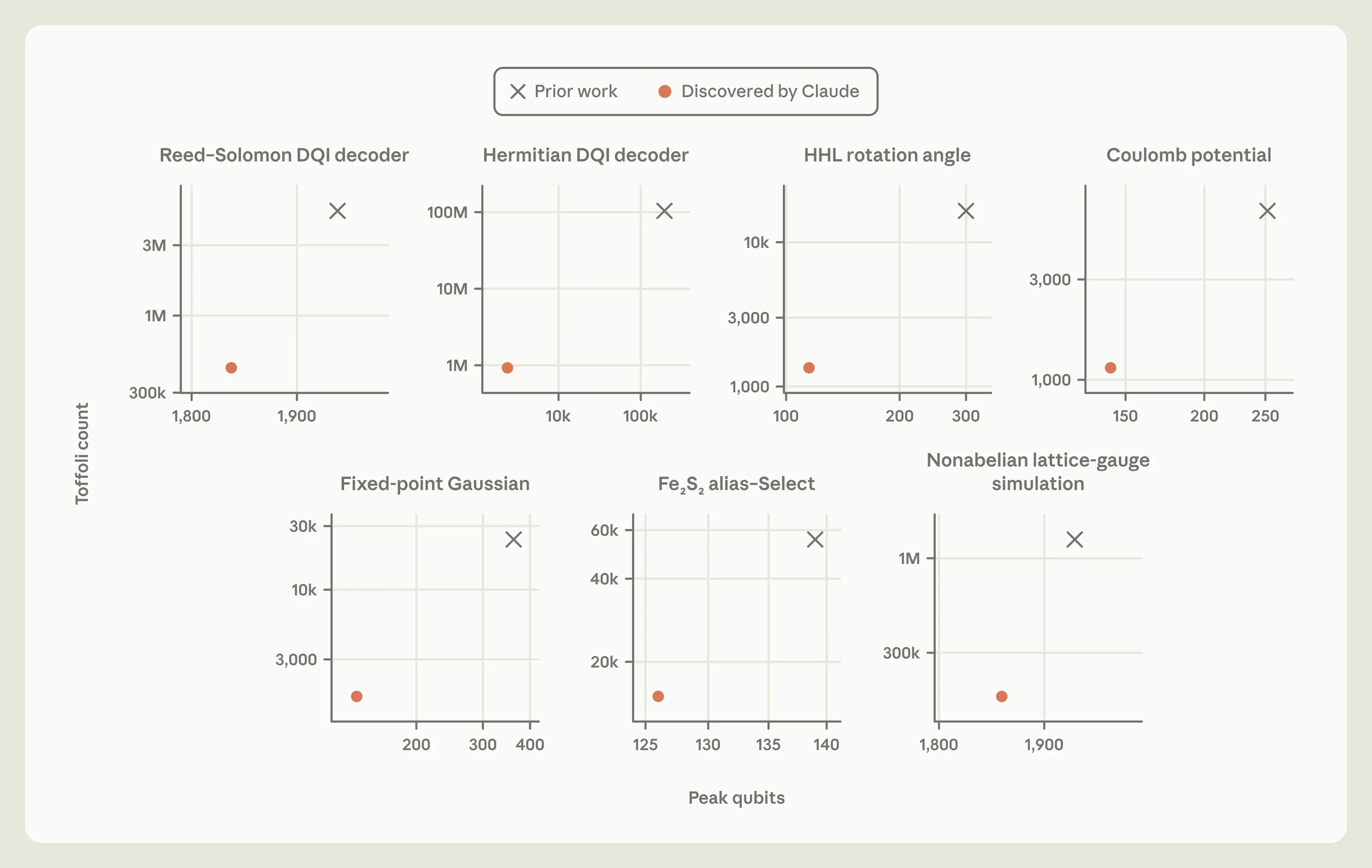
Figure 2: Claude designed smaller and faster circuits across eight different quantum-circuit design tasks. Gray marks show the best previously published designs; orange marks and lines show Claude’s designs. Point addition, the eighth task, is compared in Table 1 below.

A new reversible algorithm

Designing a quantum circuit involves two constraints that ordinary programming doesn’t have. The first is that a quantum circuit can’t make “if-then” decisions the way an ordinary program can. An ordinary program can check a value and then run only one of two pieces of code. But a quantum computer runs on a superposition of many inputs at once, some of which would run the first piece of code and some of which would run the second, so the circuit has to include the operations for both every time it runs.

The second is that a quantum circuit can’t discard information. An ordinary program can overwrite or delete its scratch work once it’s completed it; in a quantum computer, such intermediate information can’t simply be erased, because every step of a quantum circuit must be reversible. Leaving that information in place isn’t an option, either, because leftover scratch work would corrupt the final result. The only way to discard information is to “uncompute” it by running the computation that created it in reverse, at the cost of additional gates. Both of these constraints make quantum circuits far more expensive, in both runtime and qubits, than their classical counterparts.

This constraint forces a difficult trade-off between space (i.e., qubits) and time. At one extreme, a quantum circuit can uncompute intermediate results as soon as they have been used. This frees up qubits, but if those same results are needed again later, the circuit must recompute them, which adds gates and increases the runtime. At the other extreme, the circuit can retain intermediate results until they’re no longer needed. This avoids repeating work, but it can require many more qubits.

This is what makes quantum circuit design an especially interesting test of Claude’s capabilities. The circuits can be written as ordinary code, but improving them requires the model to reason under a set of constraints quite unlike those of ordinary programming.

A hard first test: modular inversion

The first task we gave Claude was point addition, a rule for combining two points on a mathematical curve (an elliptic curve) to produce a third. Point addition is the core step in quantum algorithms for the discrete logarithm problem on elliptic curves: given a starting point and the result of adding it to itself n times, find n. For large curves, ordinary computers can’t solve this problem in any reasonable amount of time, but a sufficiently large quantum computer could.

These algorithms perform point addition many times over, including in reverse, and these additions account for most of their qubit and runtime costs. Problems like this—easy to compute, extremely hard to reverse—were among the first where quantum computers were shown to offer an exponential speedup over ordinary ones. For these reasons, point addition has become one of the field’s standard benchmarks. This made it a demanding test for Claude. So, we asked it to map out how few qubits, as well as how few gates, point addition really needs.

We gave Claude a one-paragraph brief. It explained the mathematical rule for point addition, and how the evaluator would check each proposed circuit for correctness and score it on the number of qubits and gates it used. It also instructed Claude to explore several approaches in parallel. After working for 53 hours with minimal human input (limited to the initial brief and occasional prompts to think more broadly), Claude arrived at a completely new approach to the problem.

The memory demands of divsteps

Most of the cost of point addition comes from a single step, called modular inversion. Elliptic-curve arithmetic uses numbers that wrap back around when they reach a fixed limit. Modular inversion is the wraparound version of division: given an integer a, find x such that ax ≡ 1 (mod p). Ordinary computers can perform this operation efficiently using a method called divsteps. Divsteps starts with a pair of numbers and repeatedly simplifies them over many rounds of iteration. In each round, divsteps examines the current pair of numbers and conditionally swaps, adds, subtracts, or halves them. Along the way, it preserves just enough information to produce the modular inverse at the end.

Despite its success on ordinary computers, divsteps had not yet produced a practical quantum circuit, because of the reversibility constraint described above. The record of which operation was chosen at each iteration, called branch information, is the kind of scratch work that a traditional program can simply discard. In contrast, a quantum circuit has to retain that record so the computation can be run backward. A straightforward quantum version of divsteps is therefore forced to accumulate a long history of branch information, which requires an enormous number of additional qubits to store.

How Claude got around the memory problem

Claude recognized that this divsteps approach could be promising for quantum circuits, but only if there were a way around needing to store the full history. It had an idea: perhaps the record didn’t need to be stored at all. Claude reasoned that it might be possible to directly infer (or “decode”) the branch information by carefully inspecting the pair of numbers after each iteration. In essence, the numbers themselves would store the record. The circuit could then be run backward without needing any extra qubits.

To test this idea, Claude explored a number of simple candidate rules for performing the decoding. These early rules worked on small test cases, but they failed when Claude tested them at the full problem size, on 256-bit numbers.

Claude then tried a more theoretical approach. Rather than guessing and testing rules, it set out to understand mathematically why divsteps behaves the way it does. It proved a series of results about the iteration process, including several new algebraic identities. From these identities, Claude derived a precise formula for the decoding rule that would correctly recover the branch information from the numerical pairs. It then checked the formula, first by running it through large-scale numerical simulations, and then formalizing the claim in Lean. With the full validation complete, Claude produced the first reversible implementation of divsteps with no stored branch history.

A family of designs

Decoding saves qubits, but it costs time. So, as a further refinement, Claude looked for situations in which it would be cheaper to store the branch information than to decode it. By varying the threshold at which the circuit stores rather than decodes the branch information, Claude produced a new family of designs between the two extremes. Compared with the smallest previous design, one circuit in the family uses 12% more qubits but 17x fewer gates. More generally, the new designs expand the Pareto frontier, offering combinations of qubit count and runtime that weren’t available before (Table 1).

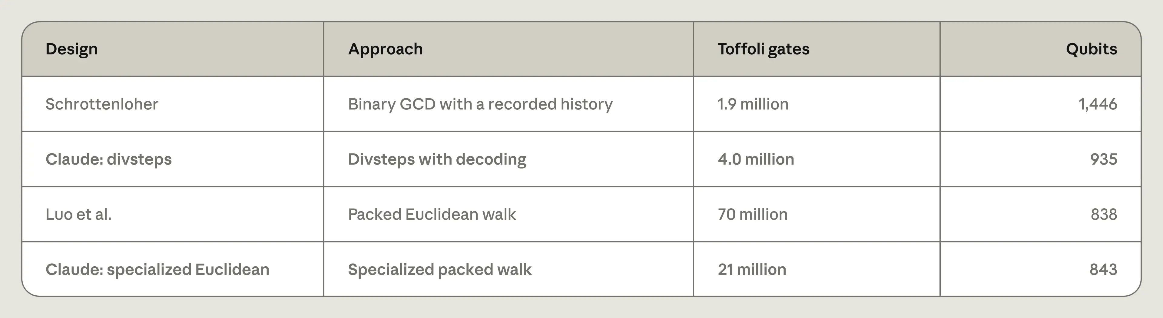
Table 1: Resources for elliptic-curve point addition. Bold rows are Claude’s designs; the others are the best previously published designs. Sources: Schrottenloher (2026), Luo et al. (2026).

Optimizing a quantum optimizer

Optimization problems are at the heart of a wide range of tasks, including scheduling, logistics, and materials design. An optimization problem presents a set of competing constraints and asks for the solution that satisfies as many of them as possible. Many quantum algorithms have been proposed for problems like these, but most promise only modest or uncertain gains over ordinary computers. Decoded quantum interferometry (DQI) is one of the strongest candidates for offering a _superpolynomial quantum speedup—_an advantage that rapidly widens as the problems get larger.

When a quantum computer finishes a computation, reading out its qubits produces just one answer, selected at random from the possibilities they were holding in superposition. DQI works by preparing a quantum state in which good solutions are more likely to be read out than bad ones. Doing this involves using an error-correcting decoder, which recovers a short list of “errors” from a compact summary. This is the most expensive step in the algorithm. So, if we could make a faster decoder, we could also perform DQI faster.

A more efficient quantum decoder

The researchers who introduced DQI demonstrated it on a problem called optimal polynomial intersection (OPI), a grid-based version of curve fitting (Figure 3). Imagine a grid in which each position x contains several acceptable values of y. The goal is to find a simple curve (a low-degree polynomial) that passes through an acceptable square for as many x positions as possible. DQI tackles this optimization problem using a specific type of decoder, called a Reed–Solomon decoder.

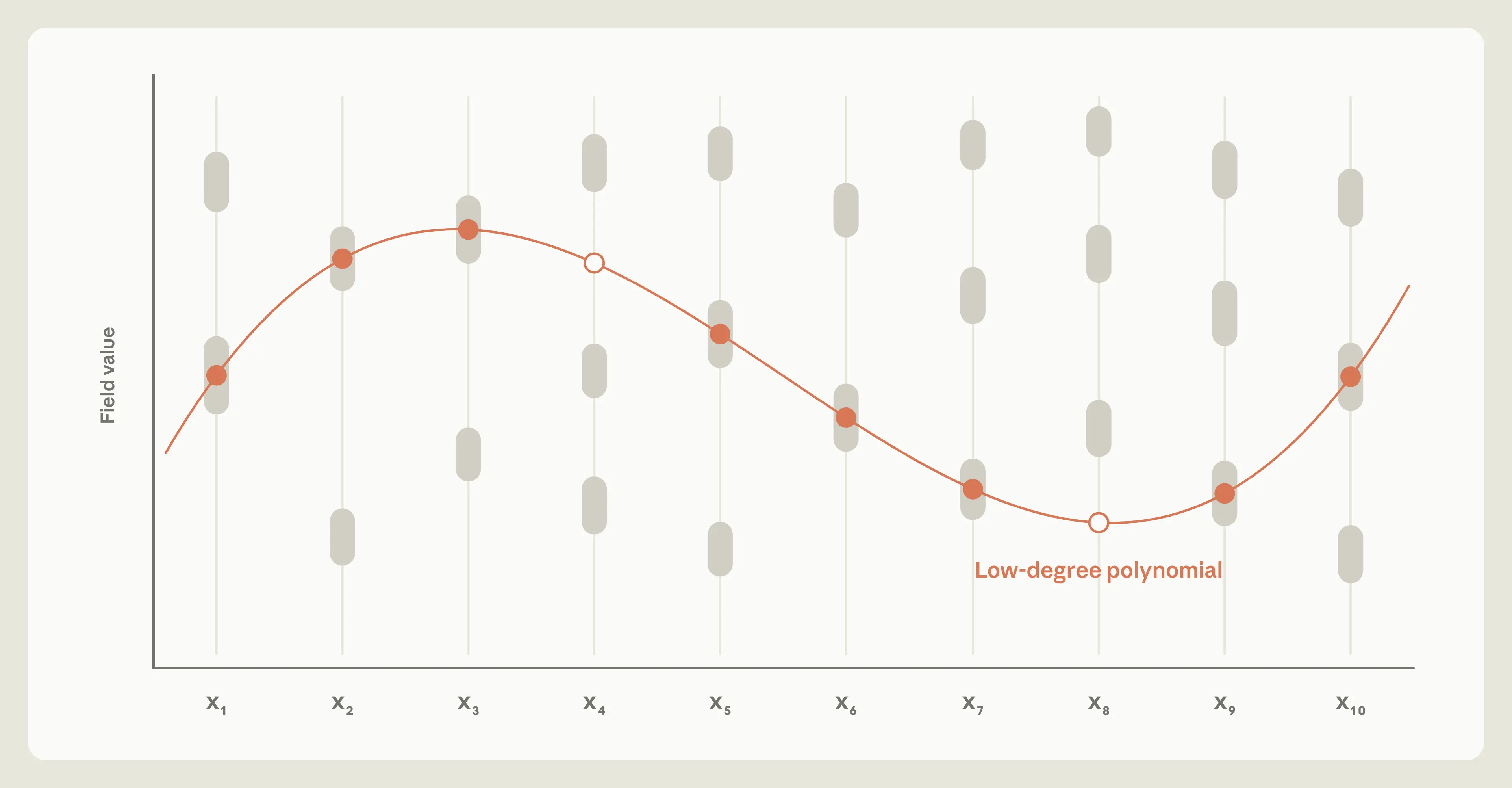
Figure 3: Optimal Polynomial Intersection (OPI) as discrete curve fitting. Each column contains several acceptable values. The optimization problem is to find a polynomial that passes through as many of the acceptable values as possible.

Reed–Solomon decoding starts from the compact summary of errors mentioned above, which is known as a syndrome. The decoder’s job is to infer, from this summary, where in the data the errors occurred and what they were. The previous state-of-the-art quantum circuit processed these syndromes using the extended Euclidean algorithm, a sequence of divisions and swaps in which the number and order of steps depend on the particular input it’s given. Here, the constraints of quantum circuits reemerge: while an ordinary program can follow a different path for every input, a quantum circuit, working on many inputs at once, has to handle all of them with a single fixed sequence of gates. To manage this, the previous design had to stretch the computation over many more rounds of iteration than any single input would need, and had to run every operation in every round, even when doing so was unnecessary.

Improving this decoder could substantially reduce DQI’s runtime. Estimates by researchers at Google Quantum AI imply that solving one particular OPI problem would take about three months on Frontier, one of the world’s most powerful supercomputers, compared with roughly an hour on a future quantum computer running DQI. Most of that hour would be spent on Reed–Solomon decoding.

So, we asked Claude to design a more efficient quantum circuit for the decoding step. Claude quickly concluded that the extended Euclidean algorithm was a poor fit for a quantum circuit. Instead, it organized its circuit around a different decoding method, known as Berlekamp–Massey decoding, which reads through syndromes (summaries of errors) one at a time and gradually works out the simplest rule that predicts each number in the list based on the ones that came before it. Once that rule is found, it reveals the errors. Unlike the extended Euclidean algorithm, Berlekamp–Massey performs the same kind of step in every round and always runs the same number of rounds, which suits a quantum circuit’s single fixed sequence of gates, ultimately giving Claude a much more efficient foundation to build on.

A simplified approach to storage

Switching to Berlekamp–Massey removed the need for the circuit to take different paths for different inputs. But making it reversible introduced another challenge, this time as a result of the uncomputing constraint discussed above. In every round, the circuit calculates temporary values that it needs only briefly, but this information can’t simply be deleted: to uncompute it later, the circuit has to be able to recover that information.

Storing this information would have been prohibitively expensive. So Claude took the same kind of approach as it had for divsteps: it found a way to reconstruct most of this information from the circuit’s current state, so it didn’t need to be stored. However, a few exceptional values couldn’t be recovered in this way and had to be saved.

Setting aside enough memory for the worst possible case, in which an exceptional value arises in 35 different rounds, would take 665 qubits. Instead, Claude wrote a high-speed simulator and ran 403 million sample decodings to measure how often these exceptions actually occurred. Almost every run needed to save one value at most. So Claude’s circuit sets aside room for just one saved value, or 19 qubits. About one run in 10,000 needs more than that and fails, which is well within the error rate the task allows. These improvements replaced large, worst-case reserves with a small, fixed number of qubits and gates (Figure 4).

Together, these optimizations reduced the number of gates in the decoder by a factor of 12 relative to Google’s previous construction. The improvement came from redesigning the computation at three levels: a different method (replacing the extended Euclidean algorithm with Berlekamp–Massey decoding), a different circuit architecture (reconstructing temporary values instead of storing them), and a different resource budget (measuring precisely how much memory and computation the circuit really needed). No single change would have been enough on its own, but together, they make the most expensive step of DQI just a little over an order of magnitude cheaper.

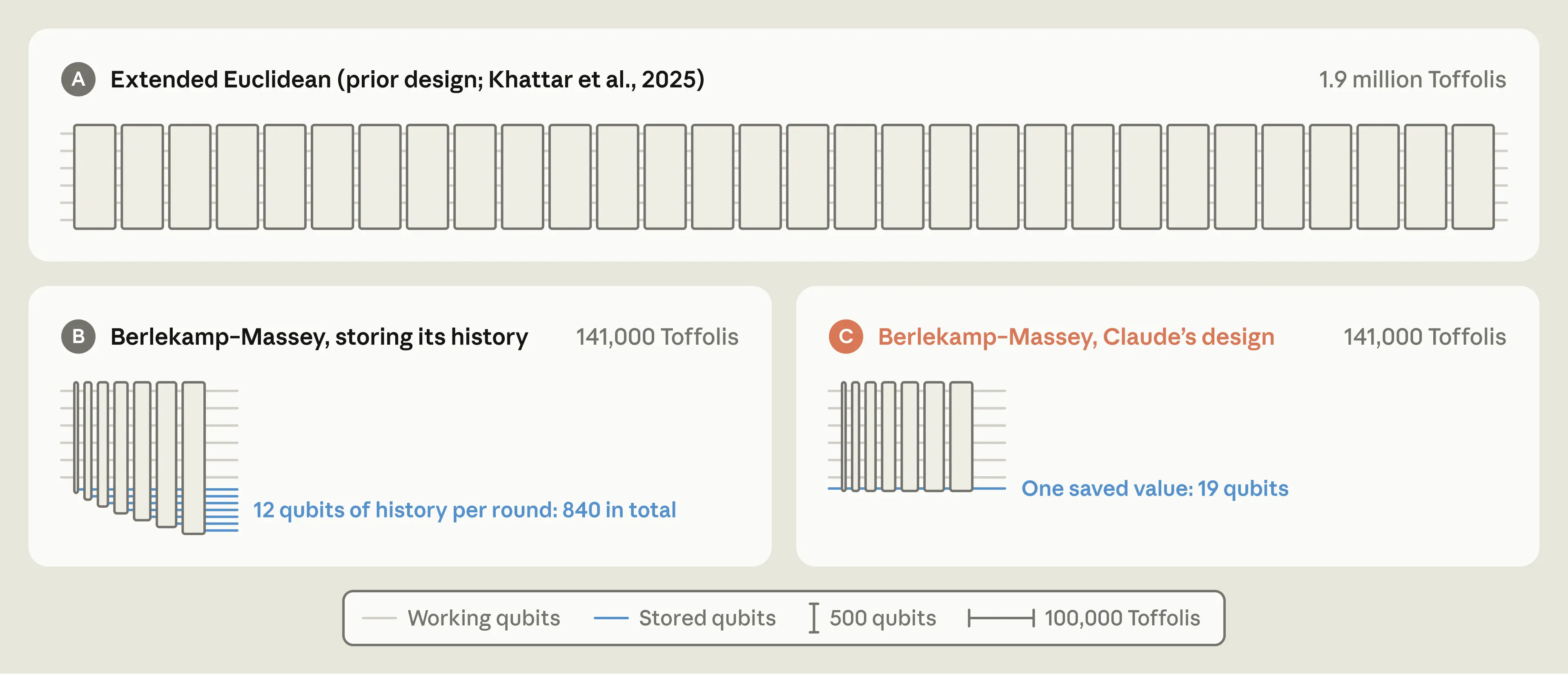
Figure 4: Three designs for the locator step of the Reed–Solomon decoder. The designs are drawn to scale: each block’s width is proportional to its gate count. (a) The previous design, based on the extended Euclidean algorithm (Khattar et al., 2025). (b) A design based on Berlekamp–Massey needs far fewer gates, but a naive reversible version has to store a 12-qubit record in every round, adding up to 840 qubits. (c) Claude’s circuit reconstructs most of the history from the updated state, so it needs to have room only for a single saved value of 19 qubits.

What we learned

Scientific progress often comes from making theoretical ideas practical. One of the main ways this happens is by making a process that was once thought to be impractical fast and cheap enough to carry out. Quantum circuit design is a prime example: the 150,000-fold drop in the FeMoco estimate described above took many research groups eight years, with each step typically representing months of work. By contrast, Claude’s elliptic-curve design was the result of a single 53-hour run.

Our results suggest that AI can support the work of circuit design, producing implementations that bring useful quantum computations closer to the capabilities of real hardware. If AI can speed up that work, useful quantum computing could arrive sooner.

Despite Claude’s encouraging performance on these tasks, we also observed some limitations. In our early experiments, Claude was conservative by nature. It repeatedly second-guessed apparent improvements, and sometimes continued to double- and even triple-check results that were already well supported. This caution was sometimes valuable: for example, it prompted Claude to write Lean proofs to verify its divsteps design. But it also manifested in a tendency to prefer existing, well-known approaches to more novel ones.

We took two steps to mitigate this. First, our setup required Claude to propose several qualitatively different approaches, and to develop them in parallel. Second, we also occasionally prompted Claude to broaden its search. These interventions succeeded in getting Claude to pursue more ambitious ideas. The elliptic-curve result, for example, didn’t come from shaving gates off of a pre-existing design but from exploring a method of doing reversible modular inversion that hadn’t been possible previously, and then deriving the mathematical results needed to make it practical. Once it had come up with the idea, Claude developed the approach, implemented it, and verified its correctness autonomously.

Circuit design is only one part of building a useful quantum computer. Because qubits are so fragile, the machine must also catch and fix its own errors as it runs, and that depends on many other components, ranging from error-correcting codes to fast decoders to control of the hardware itself. These components all affect one another, but to manage complexity, each is usually designed separately. Many of them share the characteristics that made circuit design a good fit for Claude: a design can be written as code, checked for correctness, and scored by its cost.

This raises an intriguing possibility. Rather than designing each component on its own, AI could optimize all of them jointly, from the algorithm down to the hardware, to build an entire error-corrected quantum computer tailored to a specific problem. Such designs could also tell hardware builders which capabilities matter most for a given application. That could put problems such as designing catalysts and understanding new materials within reach of the first fault-tolerant machines.

Acknowledgments

We thank Arjun Kar and Vinay Ramasesh for helpful discussions in the early stages of the project.

Feeds